MNIST 데이터셋이 있습니다. NIST(National Institute of Standards and Technology)는 필기체 인식을 위해 데이터를 수집한 것입니다. 1980년대 말에 cnn이라는 논문으로 발표를 합니다. 매우 성능이 좋은데, 딥러닝은 cnn 전후로 나눈다고 말해도 무방합니다. 미국 우체국은 손글씨를 기계를 이용해서 빠르게 분류하고 싶었다고 합니다. 이 NIST 데이터셋에서 숫자들만 모아놓은 것이 MNIST 데이터셋입니다. MNIST 데이터셋은 숫자들이 그림으로 이루어져있고 28 by 28의 픽셀로 이루어져있습니다. 6만개의 훈련용 데이터셋과 만개의 실험용 데이터셋으로 이루어져있습니다. kaggle에서 받을 수도 있고, keras에서 받을 수도 있습니다.
kaggle 주소는 다음과 같습니다.
https://www.kaggle.com/oddrationale/mnist-in-csv
MNIST in CSV
The MNIST dataset provided in a easy-to-use CSV format
www.kaggle.com
원래는 딥러닝으로 처리해야하는 이미지지만, 머신러닝으로도 처리할 수 있지 않을까 해서 시작하는 강의라고합니다.
MNIST 데이터를 가져옵니다.
import pandas as pd

df_train = pd.read_csv('./mnist_train.csv')
df_test = pd.read_csv('./mnist_test.csv')

df_train.shape, df_test.shape
((60000, 785), (10000, 785))
6만개와 만개로 나뉘고 feature가 785개가 되네요...
df_train.head()
보면 label이 있습니다. label 컬럼을 빼고나면 784개의 feature가 됩니다.
import numpy as np

np.sqrt(784)
28.0
아까 이미지가 28 by 28로 되어있다고 했으므로 제대로 나오는 것을 확인할 수 있습니다.
이제 label 컬럼을 제외하고 X,y 각각 train과 test 데이터로 나눠줍니다.
X_train = np.array(df_train.iloc[:, 1:])
y_train = np.array(df_train['label'])

X_test = np.array(df_test.iloc[:, 1:])
y_test = np.array(df_test['label'])
6만개 중에서 16개만 random choice를 해보겠습니다.
import random

samples = random.choices(poplation=range(0, 60000), k=16)
samples
[19505,
21133,
49478,
33401,
53393,
11794,
39362,
49496,
30032,
47129,
12553,
42619,
58409,
55114,
25519,
25409]
어떻게 생겼는지 보려고 16개만 뽑아봤습니다.
import matplotlib.pyplot as plt

plt.figure(figsize=(14, 12))

for idx, n in enumerate(samples):
	plt.subplot(4, 4, idx+1)
   	plt.imshow(X_train[n].reshape(28, 28), cmap='Greys') #한 행은 한 줄로 되어있으므로 reshape 시킵니다.
   	plt.title(y_train[n])

plt.show()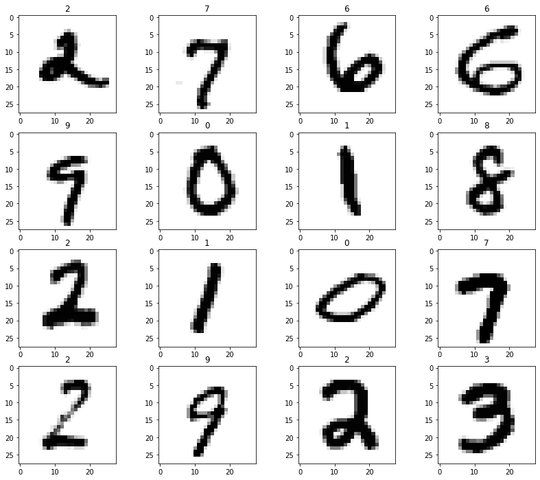
가끔 7 가운데 짝대기를 넣는 경우가 있는데 이런 경우는 참 애매하네요... 4로 볼수도 있으니까요.
from sklearn.neighbors import KNeighborsClassifier

clf = KNeighborsClassifier(n_neighbors=5)
clf.fit(X_train, y_train)
KNeighborsClassifier()
from sklearn.metrics import accuracy_score

pred = clf.predict(X_test)
accuracy_score(y_test, pred)
0.9688
784개의 feature를 가지고 있는 6만개의 데이터를 가지고 학습을 한 뒤에 만개의 데이터로 test를 하고있습니다. knn은 모든 데이터의 거리를 계산해야 하기 때문에 상당히 오래걸립니다.
따라서 pca를 통해 차원을 줄일 수 있습니다.
from sklearn.pipeline import Pipeline
from sklearn.decomposition import PCA
from sklearn.model_selection import GridSearchCV, StratifiedKFold

pipe = Pipeline([
	('pca' : PCA()),
    ('clf' : KNeighborsClassifier())
])

params = {
	'pca__n_components' : [2, 5, 10],
    'clf__n_neighbors' : [5, 10, 15]
}
params에 pipeline을 같이하면 underbar가 2개 있어야합니다.
kf = StratifiedKFold(n_splits=5, shuffle=True, random_state=13)
grid = GridSearchCV(pipe, param_grid=params, cv = kf, n_jobs=-1, verbose=1)
grid.fit(X_train, y_train)
verbose는 진행상황을 보자는 옵션입니다.
3분 6.6초정도 걸렸는데요, 저는 노트북 메모리 특성상 n_jobs=1로 바꿔서 진행해서 시간이 더 걸렸습니다. 병렬처리로 더 빠르게 진행하려면 n_jobs=-1로 두면 됩니다.
grid.best_estimator_Pipeline(steps=[('pca', PCA(n_components=10)),
('clf', KNeighborsClassifier(n_neighbors=10))])
784개의 feature를 10개로 줄였을때가 가장 좋았네요.
grid.best_score_0.9311333333333334
93점이 나오는거면 좋네요.
grid.best_params_{'clf__n_neighbors': 10, 'pca__n_components': 10}
pred = grid.best_estimator_.predict(X_test)
accuracy_score(y_test, pred)
0.9288
92.8%가 나오네요. 그리고 1분이 넘던게 3.5초만에 나옵니다. 어마어마한겁니다.
이번에는 classification report로 precision, recall f1-score, support 등을 같이 보겠습니다.
def results(y_pred, y_test):
    from sklearn.metrics import classification_report, confusion_matrix
    print(classification_report(y_test, y_pred))

results(grid.predict(X_train), y_train)
precision recall f1-score support
0 0.96 0.98 0.97 5923
1 0.98 0.99 0.98 6742
2 0.96 0.96 0.96 5958
3 0.94 0.90 0.92 6131
4 0.94 0.93 0.93 5842
5 0.93 0.94 0.93 5421
6 0.96 0.98 0.97 5918
7 0.96 0.95 0.96 6265
8 0.92 0.91 0.91 5851
9 0.90 0.91 0.90 5949
accuracy 0.94 60000
macro avg 0.94 0.94 0.94 60000
weighted avg 0.94 0.94 0.94 60000
실제 3중에서 3을 제일 못맞췄고 드르등등을 확인할 수 있습니다.
700번째 숫자를 그리고 그 숫자를 predict 해보겠습니다.
n = 700
plt.imshow(X_test[n].reshape(28, 28), cmap='Greys')
plt.show()

print('Ans :', grid.best_estimator_.predict(X_test[n].reshape(1, 784)))
print('Real :', y_test[n])
Ans : [1]
Real : 1
1을 1이라고 잘 맞췄네요.
800번째도 보겠습니다.
n = 800
plt.imshow(X_test[n].reshape(28, 28), cmap='Greys')
plt.show()

print('Ans :', grid.best_estimator_.predict(X_test[n].reshape(1, 784))) #X_test[n]이 shape이 (784,)로 되어있으므로 1, 784로 바꿔야함
print('Real :', y_test[n])
Ans : [5]
Real : 8
8을 5라고 했네요... accuracy가 94%인데 6%인것을 찾아냈네요.
틀린 데이터가 어떻게 생겼는지 확인해보겠습니다.
예측한 결과입니다.
preds = grid.best_estimator_.predict(X_test)
preds
array([7, 2, 1, ..., 4, 5, 6], dtype=int64)
이번엔 실제값입니다.
y_testarray([7, 2, 1, ..., 4, 5, 6], dtype=int64)
참값과 예측값이 다른 값들만 추려서 저장합니다.
wrong_results = X_test[y_test != preds]
wrong_results
array([[0, 0, 0, ..., 0, 0, 0],
[0, 0, 0, ..., 0, 0, 0],
[0, 0, 0, ..., 0, 0, 0],
...,
[0, 0, 0, ..., 0, 0, 0],
[0, 0, 0, ..., 0, 0, 0],
[0, 0, 0, ..., 0, 0, 0]], dtype=int64)
wrong_results.shape[0]712
712개가 틀렸다고 나오네요.
samples = random.choices(population=range(0, wrong_results.shape[0]), k=16)틀린 데이터 총 개수중에서 16개만 가져와보자는 뜻입니다.
plt.figure(figsize=(14, 12))

for idx, n in enumerate(samples):
    plt.subplot(4, 4, idx+1)
    plt.imshow(wrong_results[n].reshape(28, 28), cmap='Greys')
    pred_digit = grid.best_estimator_.predict(wrong_results[n].reshape(1, 784))
    plt.title(str(pred_digit))

plt.show()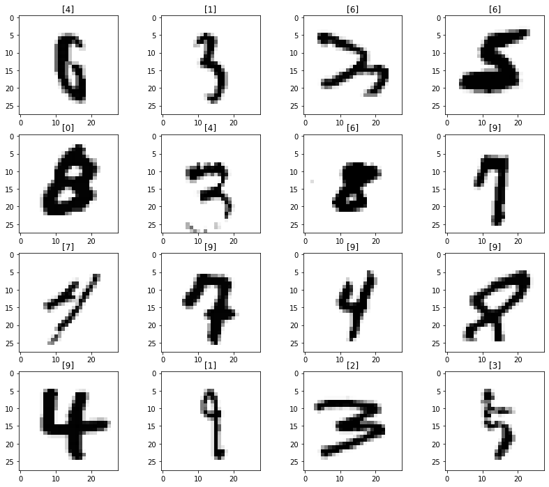
틀릴만한 것들도 꽤 많네요...
'머신러닝 > PCA(Principal Component Analysis)' 카테고리의 다른 글
| 비지도학습 (Clustering) (0) | 2024.06.05 |
|---|---|
| HAR using PCA (0) | 2024.06.04 |
| PCA - eigenface (0) | 2024.06.01 |
| PCA - wine 데이터 (0) | 2024.06.01 |
| PCA - iris 데이터 (0) | 2024.06.01 |


